1. Motivation of the benchmark
Figure out how different algorithms in various solvers perform.
2. Benchmark cases
Gehring & Homberger vrptw 200, 600 cases
3. Solver options
| solver | initial solution algo | heuristic | # threads |
|---|---|---|---|
| ortools | Christofides (chris) | gls, sa, gts* | 1 |
| ortools | Path Cheapest Arc (pca) | gls, sa, gts | 1 |
| ortools | Savings | gls, sa, gts | 1 |
| ortools | ensemble** | gls, sa, gts | 1 |
| jsprit | default | default | 1, 2, 8 |
*Heuristic names: guided local search (gls), simulated annealing (sa), genetic tabu search (gts)
**ensemble: Using saving algorithm to quickly get an estimated number of routes, then use it as van count and use pca for initial solution
4. Results
We first compare the performance of solver options by performance profile (PP). Each plot in one PP shows the performance of one solver option. It indicates how many problems can be solved to what optimality, where x-axis (tau value) is the cost multiplier to optimal solution. For example, a point (1.05, 0.8) in a PP represents the solver solves 80% of problems to at most 5% optimality gap to the best solutions. All solver options are set to use consistent runtime, which may vary based on order size of problems.
| # nodes | 10 | 20 | 50 | 70 | 100 | 150 | 200 | 300 | 400 | 500 | 500+ |
|---|---|---|---|---|---|---|---|---|---|---|---|
| runtime limit(s) | 0.5 | 1 | 2 | 4 | 7 | 20 | 30 | 60 | 140 | 200 | 270 |
4.2 Gehring & Homberger cases
Notes that for jsprit, only try running with 8 threads. Otherwise, the gap will be huge.
For C1 cases,
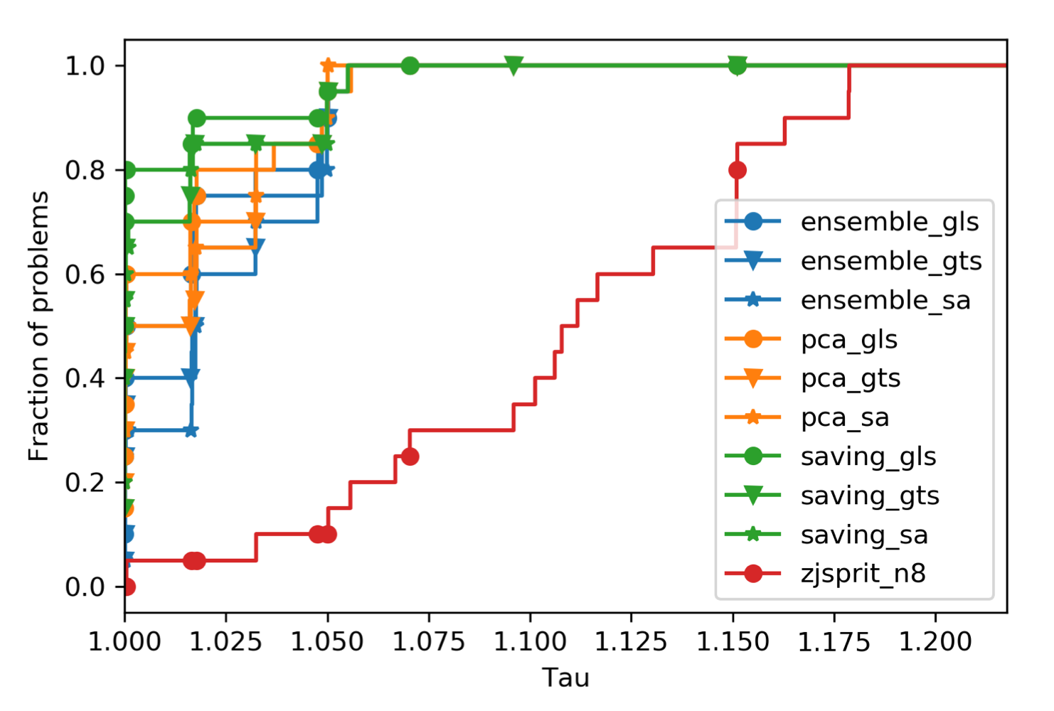
For C2 cases,
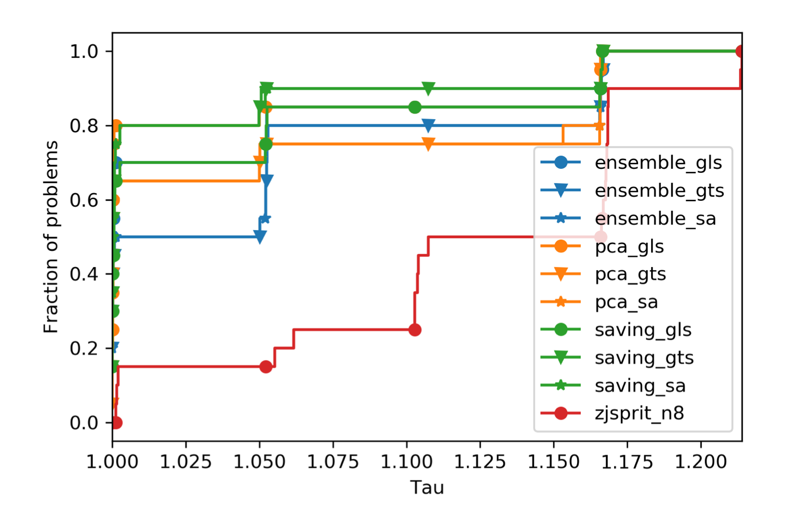
For R1 cases,
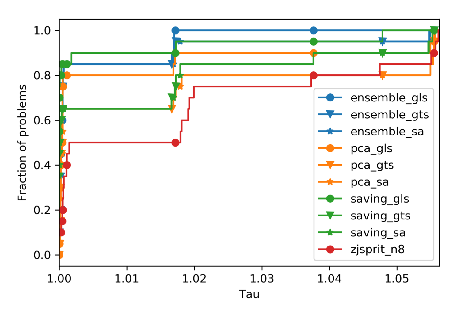
For R2 cases,
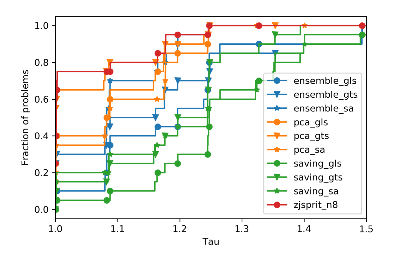
For RC1 cases,
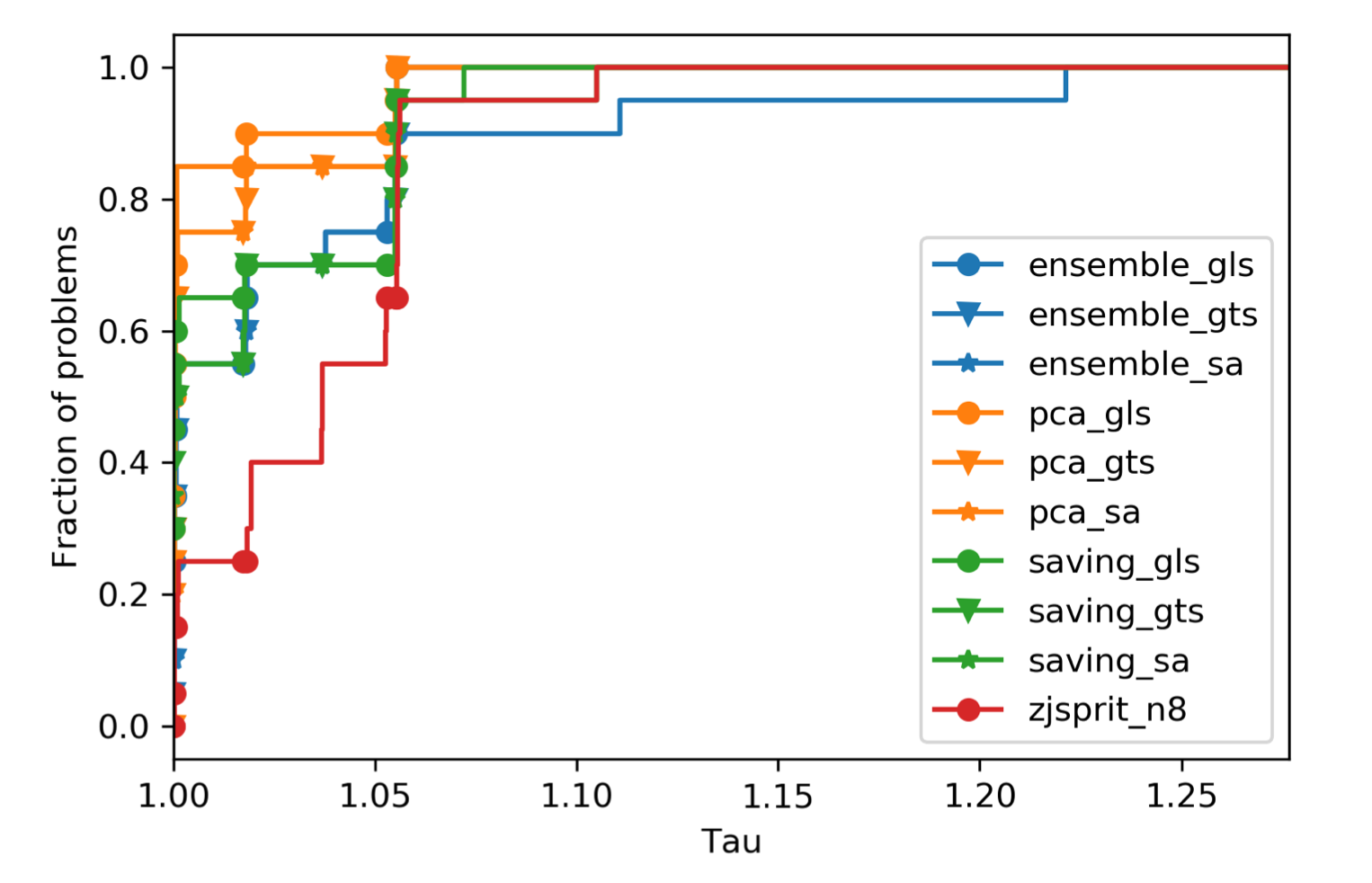
For RC2 cases,
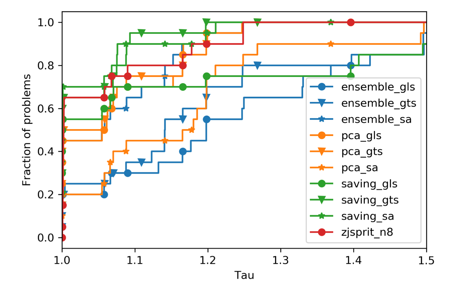
Observations:
- For R2 and RC2 cases, ortools are relatively weak. In these two categories, van capacities are larger, time window of orders are wider, order locations are not clustered.
5. Solver combination
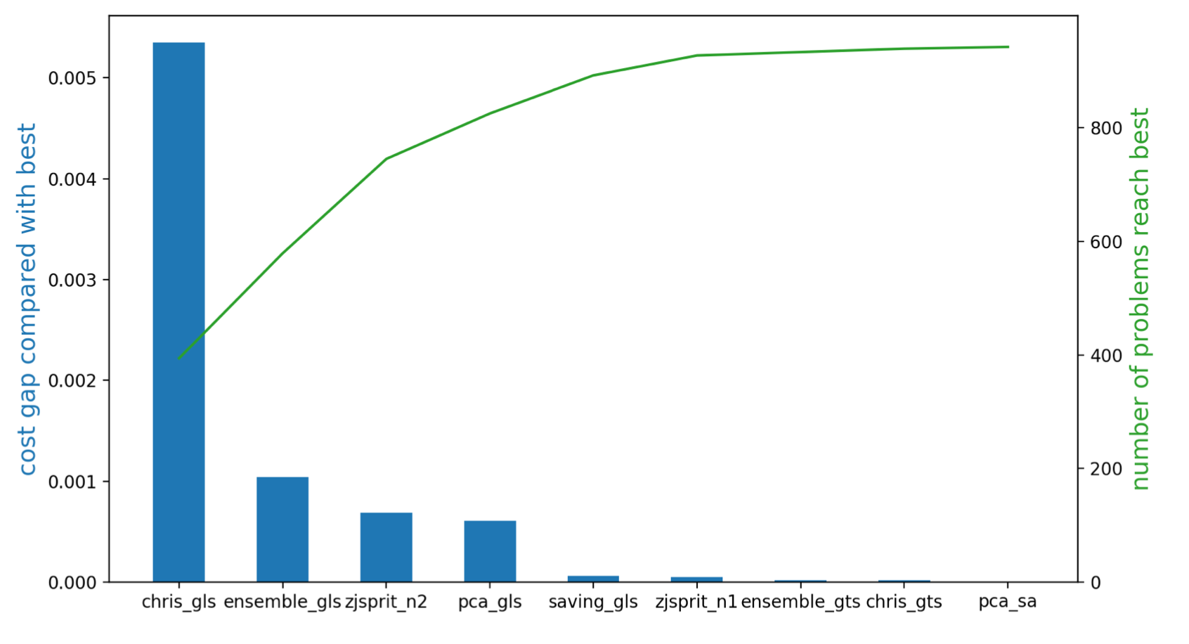
Based on above results, now we try to decide the priority of solvers. Notice that here we only consider Walmart cases. We start from empty solver set. Then do the following iterations: For each iteration,
- Compute the number of problems that each solver can reach to the best solutions
- Choose the solver which leads to the largest ns, put it into solver set
- remove problems that the chosen solver reaches the best solutions So in each iteration, we choose one solver into the solver basket. The below figure shows the number of problems that the solvers in solver basket can solve to the best, as well as the cost gap to optimality.
